Why NERC PRC-029-1's "3-6 cycles" may say more about yesterday's methods than today's capabilities
1. Introduction: When Frequency Cried Wolf
In August 2024, engineers at ERCOT's IBR Working Group presented an uncomfortable finding from the Odessa 2022 disturbance: the measured rate of change of frequency (ROCOF) during fault clearing had exceeded 5 Hz/s — well above the threshold that triggers automatic IBR disconnection. The actual system frequency never came close to that excursion. The measurement was wrong. The grid was not in distress. But any inverter-based resource with ROCOF protection set at that threshold would have tripped — correctly following its settings, and incorrectly disconnecting from a system that needed it. [1]
Three separate 138 kV faults in South Texas between November 2023 and January 2024 told the same story from a different angle. Voltage angle jumps during fault clearing caused IBR trips that had nothing to do with actual system frequency behavior. Protection settings were subsequently disabled or raised at affected facilities — a workaround that addressed the symptom but not the cause. [2]
At the center of both events is a question power engineers rarely ask explicitly: what does it actually mean to measure frequency at a bus terminal, and how long does it reliably take?
NERC PRC-029-1 [3] — the new inverter-based resource performance standard effective 2025 — contains a deceptively simple answer in Attachment 2, page 14:
"Frequency is measured over a period of time (typically 3-6 cycles) to calculate system frequency at the high-side of the main power transformer." [3, Attachment 2, Item 2]
Immediately following:
"Instantaneous or single points of measurement may not be used in the determination of control settings." [3, Attachment 2, Item 3]
With compliance deadlines now in force and hundreds of IBR projects in interconnection queues across North America, these two sentences are being embedded in protection relay settings industry-wide. Yet the Odessa and South Texas events expose the question those sentences do not answer: is "3-6 cycles" the right constraint — or does it describe the limitations of methods that were standard forty years ago?
This article explores the physics and mathematics of frequency estimation, surveys the evolution of methods from zero-crossing to spectral and geometric estimators, and ends with a provocation: is it time for NERC standards to specify what accuracy frequency protection must achieve, rather than how many cycles it must observe?
2. Electrical Frequency Is Always an Estimate
Power engineers rarely make one distinction explicitly: rotating frequency versus electrical frequency. It matters more than it might seem.
When a synchronous generator runs at stable speed, its shaft rotates at a mechanical frequency directly proportional to electrical frequency through the number of pole pairs — a fixed, physical relationship. An encoder on that shaft gives you something tangible to count: mechanical events per unit time. This is a measurement in the classical sense.
Electrical frequency at a bus terminal is a fundamentally different matter. No "frequency" exists as a property of the bus itself — only a voltage waveform exists, sampled at discrete intervals. Frequency must be inferred from that waveform. As Boashash established in his foundational 1992 paper, instantaneous frequency (IF) has physical "meaning only for monocomponent signals, where there is only one frequency or a narrow range of frequencies varying as a function of time" [4]. However, a real power system voltage — carrying harmonics, noise, transients, and imbalance — is not a monocomponent signal. Its instantaneous frequency is not a well-defined single value.
In these circumstances, the estimated frequency is a mathematical construct that does not map directly to physical rotation. Federico Milano et al. catalogued five known paradoxes of instantaneous frequency [5]. The most practically important: an instantaneous frequency estimator can report values outside the physical spectral band of the signal during transients — meaning a relay could report 61.5 Hz at a bus where the true fundamental has never left 59.9 Hz.
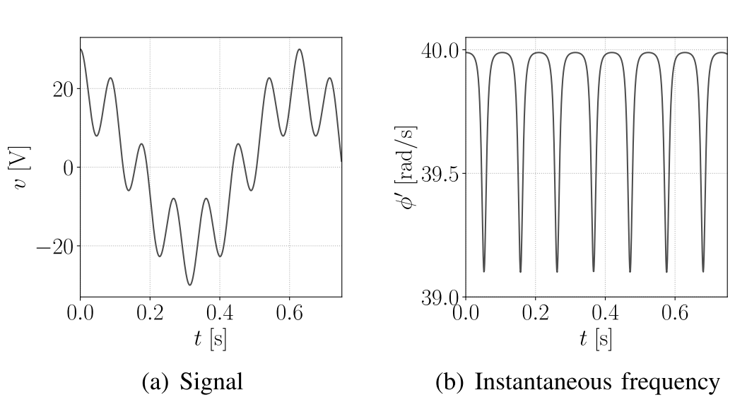
Electrical frequency at a bus terminal is always an estimated quantity. Every relay, every PMU, every IBR control loop produces not a measurement but an inference drawn from a sampled waveform. The rotating machine gives you something to measure; the bus terminal gives you something to estimate, with its inherent limitations and uncertainty.
3. Electrical Frequency Estimation Methods
Three families of methods dominate in practice — and they differ more than most relay datasheets suggest.
3.1. Classical Methods: Zero-Crossing and Its Limits
The simplest approach to frequency estimation is zero-crossing detection: identify the moments when the voltage waveform crosses zero, measure the time T/2 between successive crossings at each phase, and compute f = 1/T by averaging across all three phases.
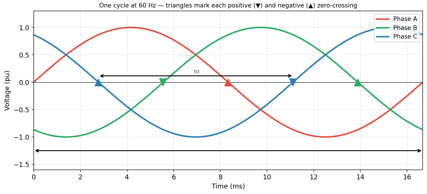
For single-phase systems, this yields one period estimate per half-cycle — two per full cycle. For three-phase systems, six zero-crossings occur per cycle (one per half-cycle per phase), theoretically providing six period estimates per cycle and enabling faster averaging. In balanced conditions, the three phases can be cross-checked for consistency; in unbalanced or distorted conditions, each phase may carry different harmonic content, complicating the choice of which crossings to trust.
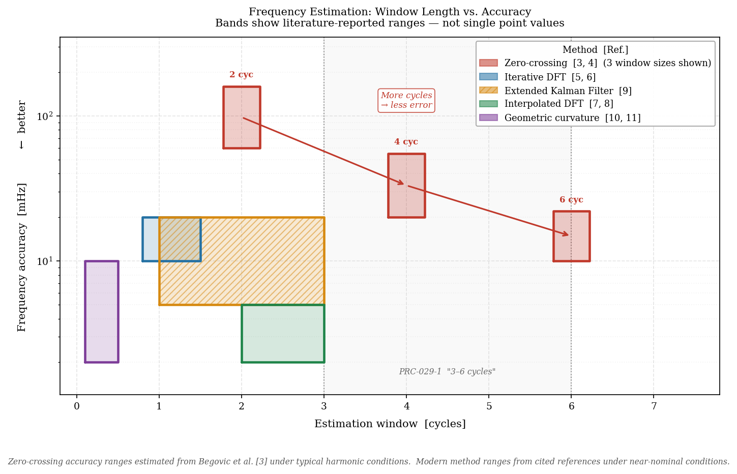
The vulnerability is harmonic content. Even modest harmonic distortion creates false zero-crossings — points where the distorted waveform crosses zero between the fundamental's true crossings — or shifts the apparent timing of real crossings. Begovic, Djuric, Dunlap, and Phadke (1993) demonstrated that zero-crossing detection is materially degraded by harmonic content at levels routinely present in distribution and industrial systems. [6] Low-pass pre-filtering mitigates this, but introduces additional group delay.
Post-processing techniques — Olympic filtering (discard the highest and lowest of four period estimates, average the remaining two), IIR smoothing — add further lag. Zero-crossing-based frequency estimation needs several cycles of averaging to suppress harmonic noise to the +/-10-100 mHz level required for protection decisions.
"Zero-crossing" is not a single method but a family of implementations. At the basic end sits direct zero detection on the raw single-phase waveform; at the sophisticated end, positive-sequence voltage extraction followed by multi-cycle filtered averaging — with many variants in between. The accuracy range of +/-10-100 mHz reflects this diversity as much as it reflects a fundamental limitation. Two devices that both claim to use "zero-crossing" can behave very differently depending on which variant is running inside. Importantly, these figures apply under normal, non-event conditions — during actual grid disturbances the errors are larger and considerably harder to bound.
IEC 61000-4-30:2015 codifies this for power quality instrumentation by specifying a 10-second primary compliance window with a permitted frequency uncertainty of +/-10 mHz. [7] For protection purposes, where faster response is required, the window shrinks — but the harmonic-susceptibility problem remains.
This is the engineering reality behind the "3-6 cycles" language in PRC-029-1 [3]. It reflects the operating regime of classical zero-crossing methods. The standard codifies a reasonable constraint for this class of methods. The critical question is whether that constraint should apply universally, regardless of what method is actually being used.
3.2. Modern Methods: Trading Cycles for Complexity
The past four decades have produced a progression of frequency estimation algorithms that offer better accuracy, faster convergence, or both — at the cost of greater computational burden.
DFT-based methods, pioneered by Phadke, Thorp, and Adamiak (1983) and refined through iterative and interpolated variants, apply spectral analysis to short voltage data windows. The iterative DFT (Sidhu and Sachdev, 1998) achieves 0.01-0.02 Hz accuracy in approximately one cycle at 50 Hz. More advanced interpolated variants (Derviskadic, Romano and Paolone, 2018) deliver full PMU-class accuracy — better than +/-5 mHz — using windows of just 2-3 cycles, simultaneously compliant with both P-class and M-class requirements of IEEE C37.118.1-2011. [8, 9, 10, 11, 15]
Extended Kalman Filter (EKF) estimators model the voltage waveform as a nonlinear state-space process and update frequency estimates recursively with each new sample. Dash, Pradhan, and Panda (1999) demonstrated convergence to protection-grade accuracy within 1-3 cycles, even when the signal is corrupted by noise and harmonics. [12]
Milano's geometric approach took a different route entirely: instead of processing a window of waveform samples, they compute frequency from the shape of the three-phase voltage vector as it traces a path in the complex plane — no window, no spectrum, no iteration. Under normal balanced conditions the result equals system frequency exactly. The approach also produces a built-in validity signal that flags when a frequency estimate has become unreliable — useful during fault transients when all other methods quietly produce wrong answers. [13, 14]
3.3. The Key Question: Can We Do Better Than 3-6 Cycles?
The short answer is yes. DFT-based iterative methods converge in approximately 1 cycle with 0.01-0.02 Hz accuracy. Kalman filter methods converge in 1-3 cycles. Modern IpDFT algorithms achieve full PMU compliance with 2-3 cycle windows. Protection-grade devices using these modern methods achieve frequency accuracy in the +/-2-10 mHz range — better than what classical zero-crossing methods deliver even over 5-6 cycles in the presence of harmonic distortion.
A 2-cycle DFT or Kalman estimate can be materially more accurate than a 5-cycle zero-crossing average. The window count and the accuracy are increasingly decoupled. The cycle count is a proxy for accuracy when method quality is fixed; it becomes a misleading constraint when better methods are available.
One caveat applies equally to all the accuracy figures above: they are reported under near-nominal operating conditions — stable voltage and low harmonic distortion, with no transients. During the events PRC-029-1 is actually written for — fault clearing, IBR switching, and voltage sags — every method degrades. Zero-crossing is particularly exposed: waveform distortion during a fault shifts zero-crossings in ways that post-filters cannot fully correct within the protection timeframe. There is a quiet irony in the standard: it was designed for disturbance events, but the methods it implicitly endorses have the weakest performance in events.
4. Conclusion: A Question Worth Asking
Window count and frequency accuracy are not the same thing — fifty years of published work are consistent on this point. A 2-cycle DFT can outperform a 6-cycle zero-crossing average. Modern protection-grade methods routinely achieve +/-2-10 mHz — accuracy that classical zero-crossing methods cannot reach at any window length under realistic harmonic conditions.
PRC-029-1's prohibition on instantaneous single-point measurement is sound. But "typically 3-6 cycles" is a description of one class of methods, not a performance specification. A device achieving +/-5 mHz in 1.5 cycles and a device achieving +/-50 mHz in 5 cycles are treated identically today — because the standard specifies how long to measure, not how well.
The Odessa and South Texas events are a reminder that measurement quality has real consequences. As inverter-based resources dominate new interconnections and the stakes of a false trip are measured in hundreds of megawatts, one question seems worth raising in the next revision cycle: is it time to write standards that define what accuracy to achieve, rather than how many cycles to count?